Defining and executing a Sediment Scenario
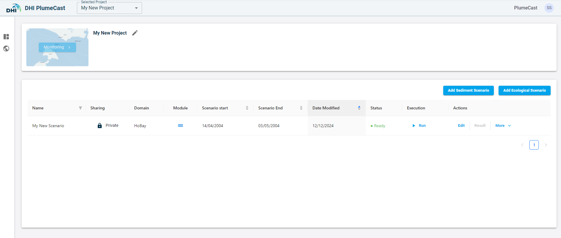
For defining a scenario, Select the project from the list of projects in Project Management Page. Click on ‘Add Sediment Scenario’ button

Scenario definition
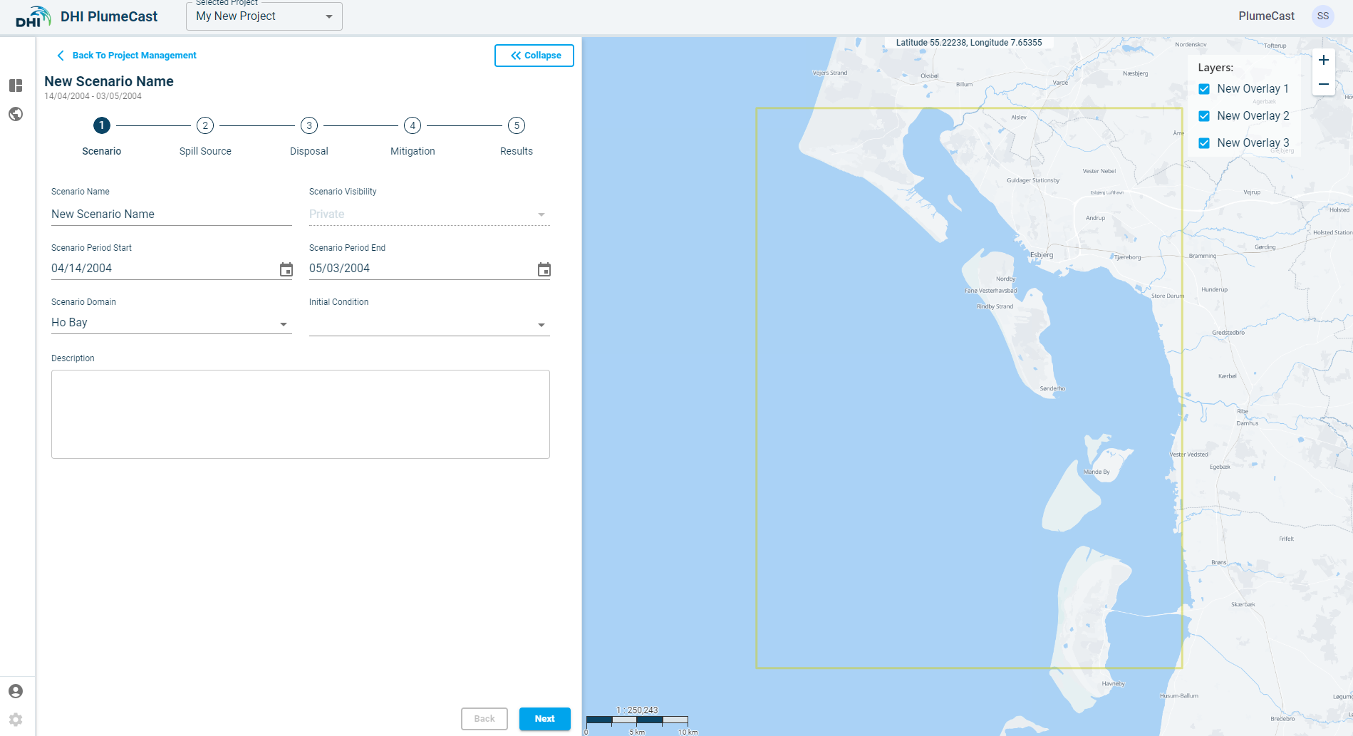
In the first step, you must give a name to the scenario. The name must be unique among other scenarios in this project.
You can choose the scenario to be ‘Private’ or ‘Shared’. ‘Private’ scenario is only visible to your user account. ‘Shared’ scenario will be visible to all other user accounts within your company.
Other DHI PlumeCast users within your company can see the scenario in their list of scenarios, but they only can see the Results. They do not have access to edit or delete the scenario.
You must select the domain from the list of available domains from the ‘Scenario Domain. The available domains correspond to the available MIKE models which have been set up and prepared for you by DHI PlumeCast administrators.
As soon as you choose the domain, the map zooms to the location of the domain. The bounding box containing the domain (in which the model is defined) are shown by a yellow rectangle on the map.
You must choose the start and end dates for the scenario. By default, they are set to the earliest and latest available dates in the chosen domain. You can choose start and end dates within this range, but not outside of it.
You can set an initial condition for your scenario. In the drop-down list, you can see a list of previously completed scenarios which have the same domain. By choosing an initial condition, the suspended sediment concentration fields and seabed deposition fields from the last time step in the chosen scenario will be used as initial conditions for the scenario you are defining now.
Finally you can add a description text for this scenario, to help noting necessary information which one should know when executing/editing this scenario.
Spill Source
The next step is to add spill sources to your scenario.
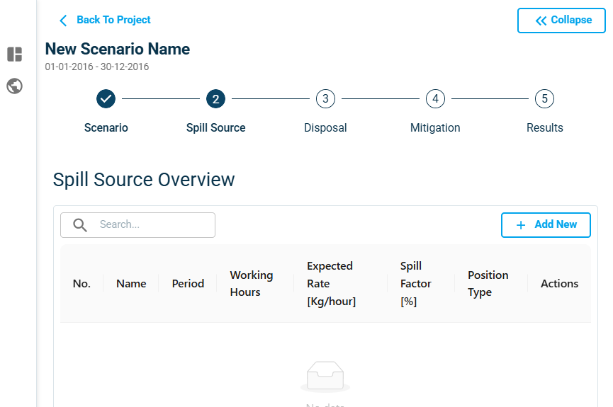
Click on ‘Add New’ button in the Spill Source step to define your spill source.
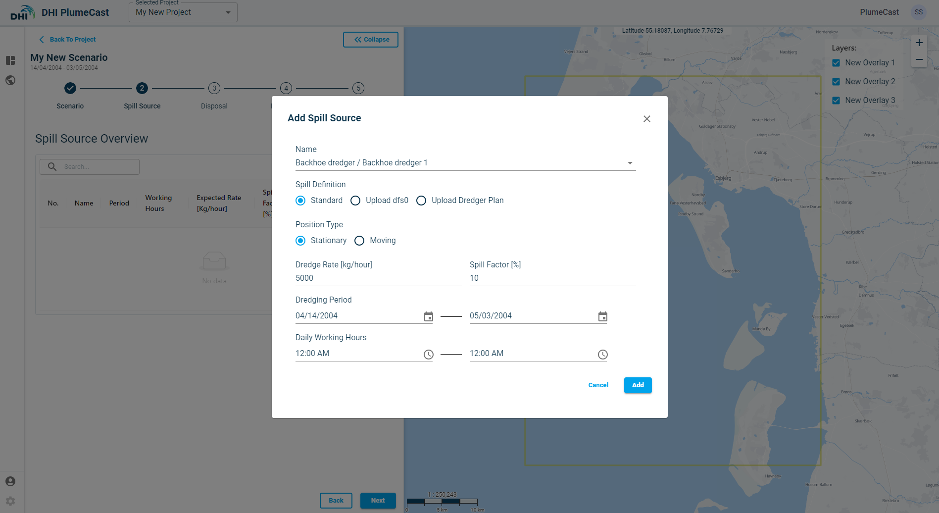
The first step is to choose the Vessel/Dredger which is producing the spill. In the drop down you can see the vessels you had defined earlier in your project.
Type of the vessel determines where in water column the spill shall be released. For example, spill from backhoe dredger is distributed uniformly in the entire water column. The spill from TSHD overflow is released close to the surface, and the spill from CSD is released close to the seabed.
The ‘Split Barge’ vessels do not appear in this list, since they are related to disposal plume calculations and are handled separately in the next step (Disposal).

Next is to choose the type of spill definition. It can be ‘Standard’, ‘from dfs0 file’, or ‘Dredge plan’ which is based on a csv file.
Standard spill source
If you choose ‘Standard’, then you must define the spill parameters manually via the website.

‘Stationary’ spill source, means that the source of sediment spill will not move throughout the scenario. You must only provide one position for the spill source.
‘Moving’ spill source, means that the source of sediment spill moves and changes positions during the scenario. You must at least provide two distinct positions for the spill source.
‘Dredge Rate’ is the rate at which the dredging takes place. It must be given in Kilograms per Hour. In ‘Standard’ spill definition, the dredge rate will remain constant throughout the entire scenario. It is not possible to give time varying dredge rate in this case. The other two options (Upload dfs0 & upload dredge plan) allow time varying dredging rate.
‘Spill Factor’ also commonly referred to as ‘Loss’, is the percentage of dredged material which is believed to be spilled into the ambient environment. It must have a value between 0 and 100.
In ‘Standard’ spill definition, the spill factor will remain constant throughout the entire scenario. It is not possible to give time varying spill factor in this case. The other two options (Upload dfs0 & upload dredge plan) allow time varying spill factor.
‘Dredging Period’ can be defined equal to the scenario period, or any other period within it.
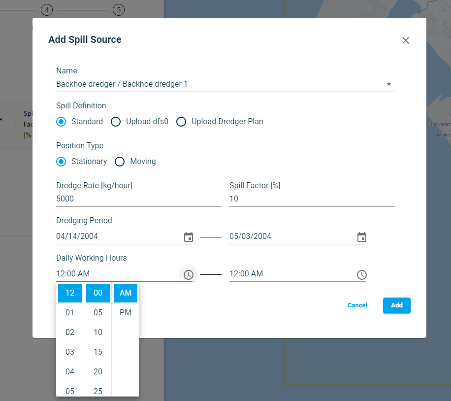
‘Working Hours’ refers to the hours dredging take place during the day. You define the daily start time and the daily end time. They will be repeated for every day during the dredging period. Select the working hours in AM or PM as required.
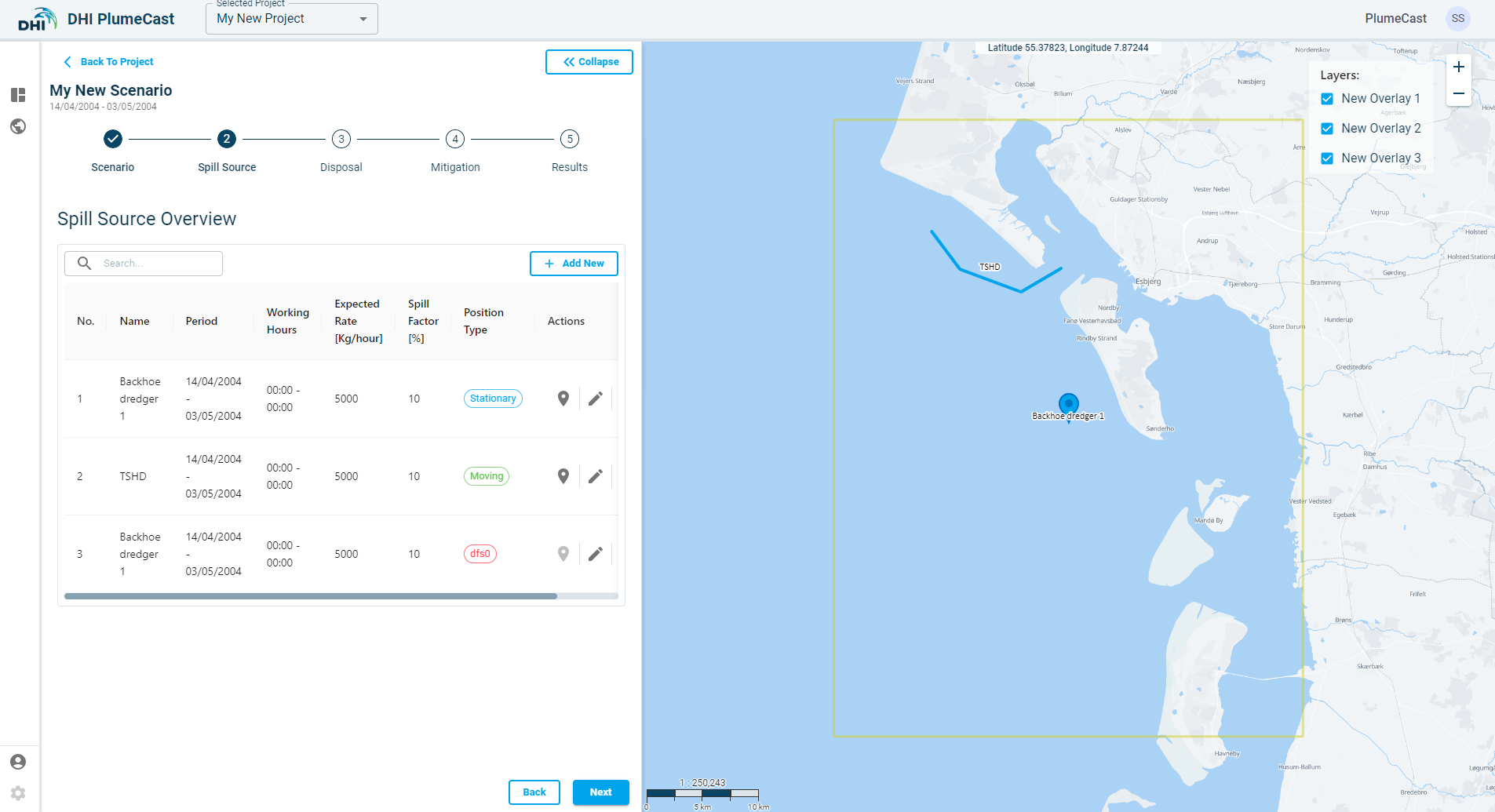
After adding the Standard Spill sources, they appear in the overview list, where you can edit them again by clicking on the ‘edit’ icon ![]() , or make a copy of them by clicking on the ‘copy’ icon
, or make a copy of them by clicking on the ‘copy’ icon ![]() .
.
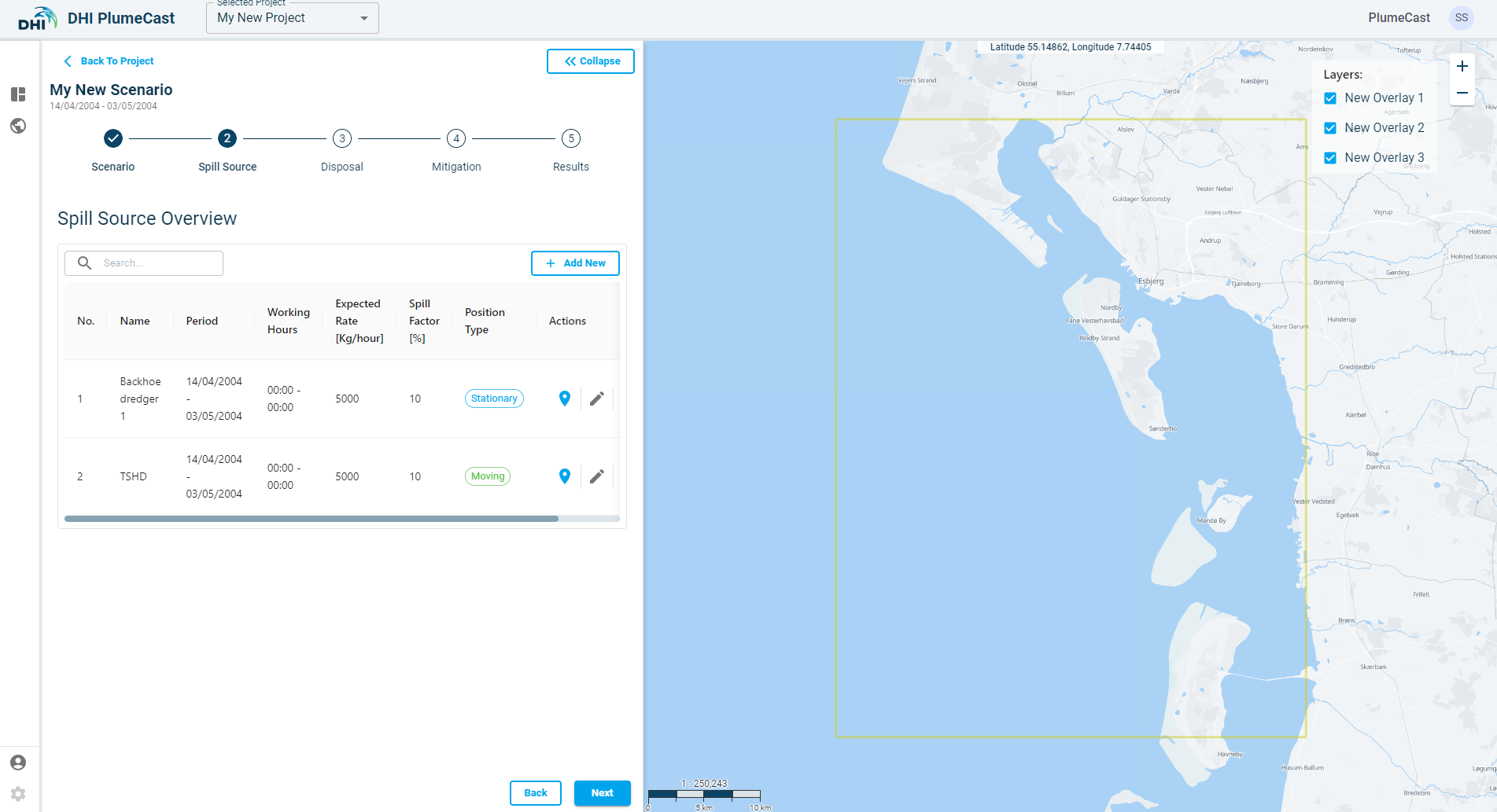
The next step is to add their location points, by clicking on the ‘location’ icon ![]() .
You cannot proceed to the next step before adding necessary number of location points to all the defined Spill Sources. To note:
• Stationary spill sources require at least one and maximum one point.
• Moving spill sources require at least two points and have no limit on maximum number of points.
• Spill source locations consist of the coordinates of the point (in Longitude & Latitude) as well as the distribution of different sediment fractions in the spill at that point.
• The number of fractions and their names and characteristics vary between different models and are defined during the model preparation stage.
.
You cannot proceed to the next step before adding necessary number of location points to all the defined Spill Sources. To note:
• Stationary spill sources require at least one and maximum one point.
• Moving spill sources require at least two points and have no limit on maximum number of points.
• Spill source locations consist of the coordinates of the point (in Longitude & Latitude) as well as the distribution of different sediment fractions in the spill at that point.
• The number of fractions and their names and characteristics vary between different models and are defined during the model preparation stage.

While in the ‘Spill Source Location’ page (above image), click on ‘Add New’. A point will be added to the list and will appear on the map. The default location of the point is at the centre of the domain borders (shown by red rectangle in the map).
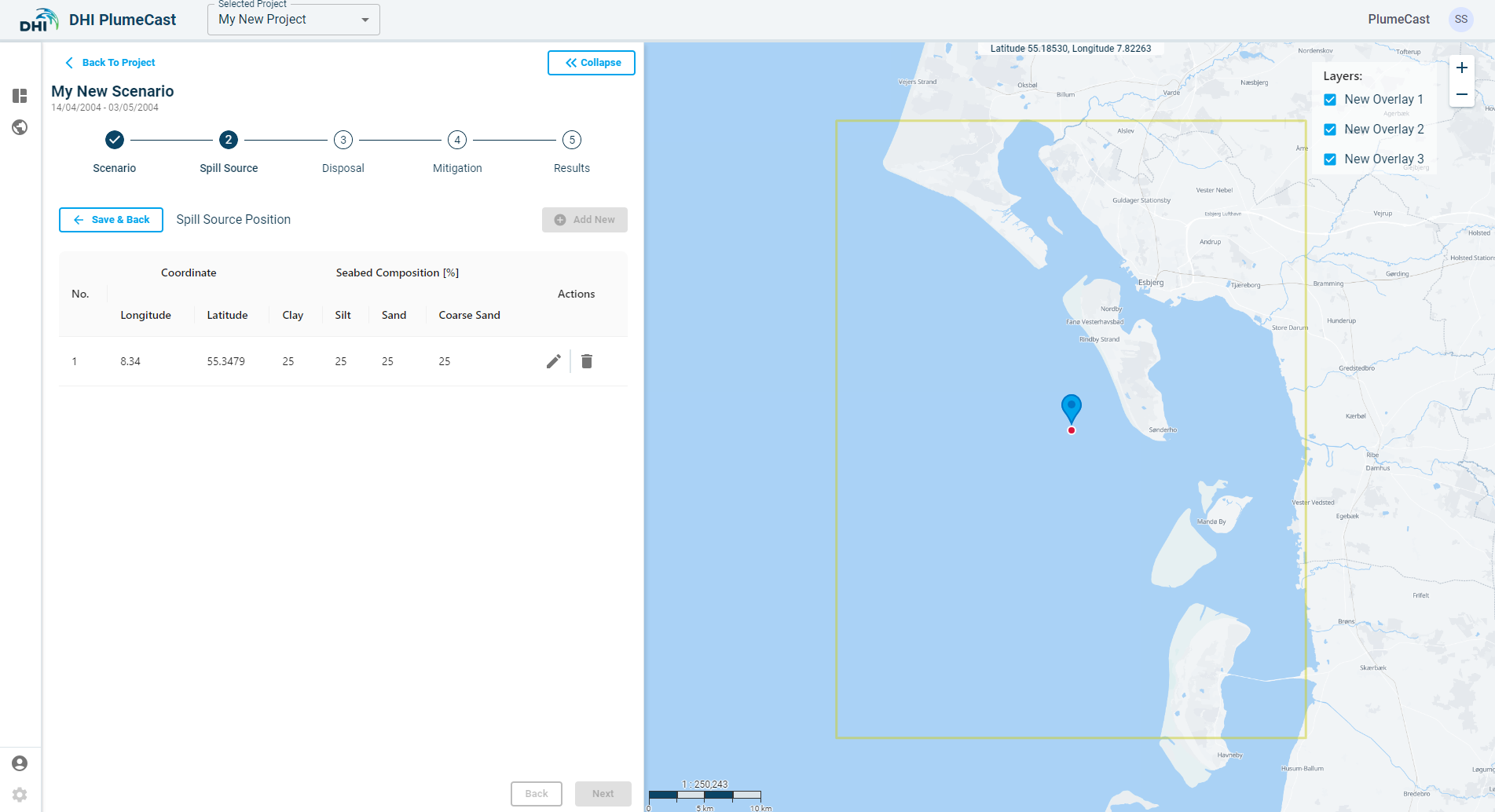
By default, all sediment fractions are given an equal share. You can change the location of the point and the distribution of sediment fractions in it by clicking on the ‘edit’ icon in front of the point in the list. *Remember that the sum of the sediment fraction percentages must always add up to 100.
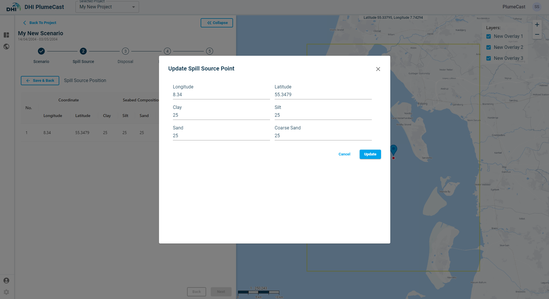
Another way to edit the location of the spill source point is by grabbing and dragging the point on the map.
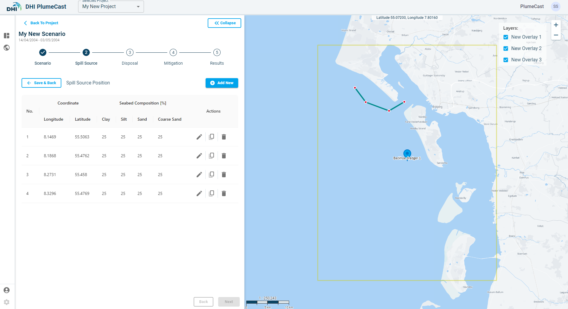
Stationary spill source only needs one point. Therefore, you cannot add more point to the list.
Moving spill source allows you to add more points to the list. It will add the next added point as continuation of the moving path. The dredger (spill source) will move with constant speed at the first point along the straight line connecting the points until the last point during the defined Dredging Period for the corresponding spill source. The distribution of sediment fractions will be interpolated between each two consecutive point with inverse distance weighting.
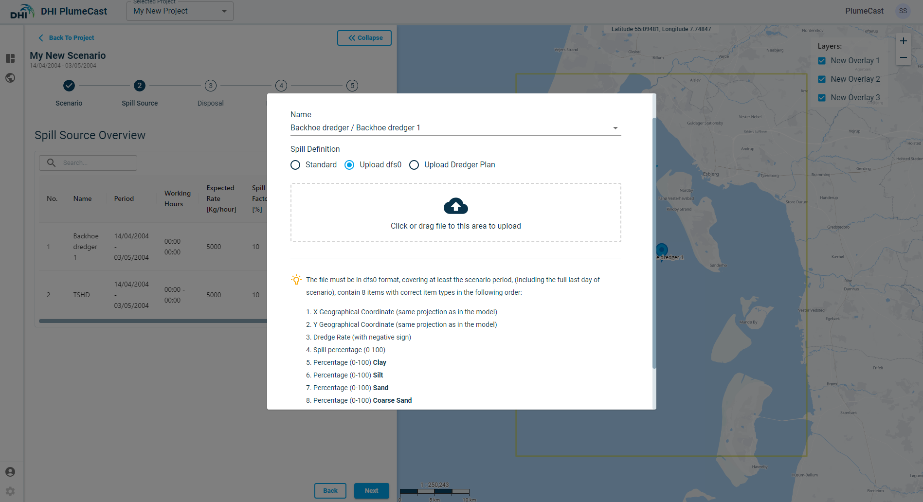
Spill source by uploading dfs0 file
If you have prepared your dredging plan in MIKE dfs0 timeseries format, you can directly upload it to DHI PlumeCast for each spill source you define in your scenario. In this case, you only need to choose the vessel. The remaining information should be present in the uploaded dfs0 file. As seen below, the dfs0 timeseries file must cover the scenario period, and have the following item types, and the number of items. In this example the domain’s sediment transport model was based on four sediment fractions, therefore the dfs0 file needs to have in total of 8 items.
If the dfs0 file is uploaded successfully, you will see a success message and clicking on ‘Add’ in the bottom right will add the file to the list. Your new spill source (with position type set to ‘dfs0’) will be added to the list of your spill sources. Currently, it is not possible to see any further information regarding the uploaded dfs0 file after being uploaded.
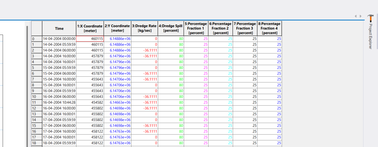
An example of a dfs0 spill source with 4 sediment fractions is shown below.
Notice that interpolation will take place between two consecutive rows. If you need to have a sharp start or stop of spillage at any time, you must introduce small time steps before/after the start/stop point, to avoid excess spillage due to interpolation. This is visible in this example:
Spill source by uploading csv format dredge plan
If you have prepared your dredging plan in csv timeseries format, you can directly upload it to DHI PlumeCast for each spill source you define in your scenario. In this case, you only need to choose the vessel. The remaining of information are supposedly delivered via the uploaded csv file.
As seen below, the csv timeseries file must cover the scenario period, and have the following columns, and the number of columns. In this example the domain’s sediment transport model was based on four sediment fractions, therefore the csv file needs to have in total of 9 columns.

If the csv file is uploaded successfully, you will see a success message and clicking on ‘Add’ in the bottom right will add the file to the list. Your new spill source (with position type set to ‘Dredge Plan’) will be added to the list of your spill sources. Currently, it is not possible to see any further information regarding the uploaded csv file after being uploaded.

An example of a csv dredge plan spill source with 4 sediment fractions is shown below. Notice that interpolation will take place between two consecutive rows. If you need to have a sharp start or stop of spillage at any time, you must introduce small time steps before/after the start/stop point, to avoid excess spillage due to interpolation. This is visible in this example:

Disposal
In this step you can define the sediment disposal events done by split-barges. In MIKE there is a specific way to calculate the spillage and deposition of disposed sediments from split-barges. It applies Nearfield calculations to identify the behaviour of the disposal plume, before inserting them into far-field.
Click on ‘Add New’ to define the Disposal Vessel and thereafter the characteristics of the disposal events.
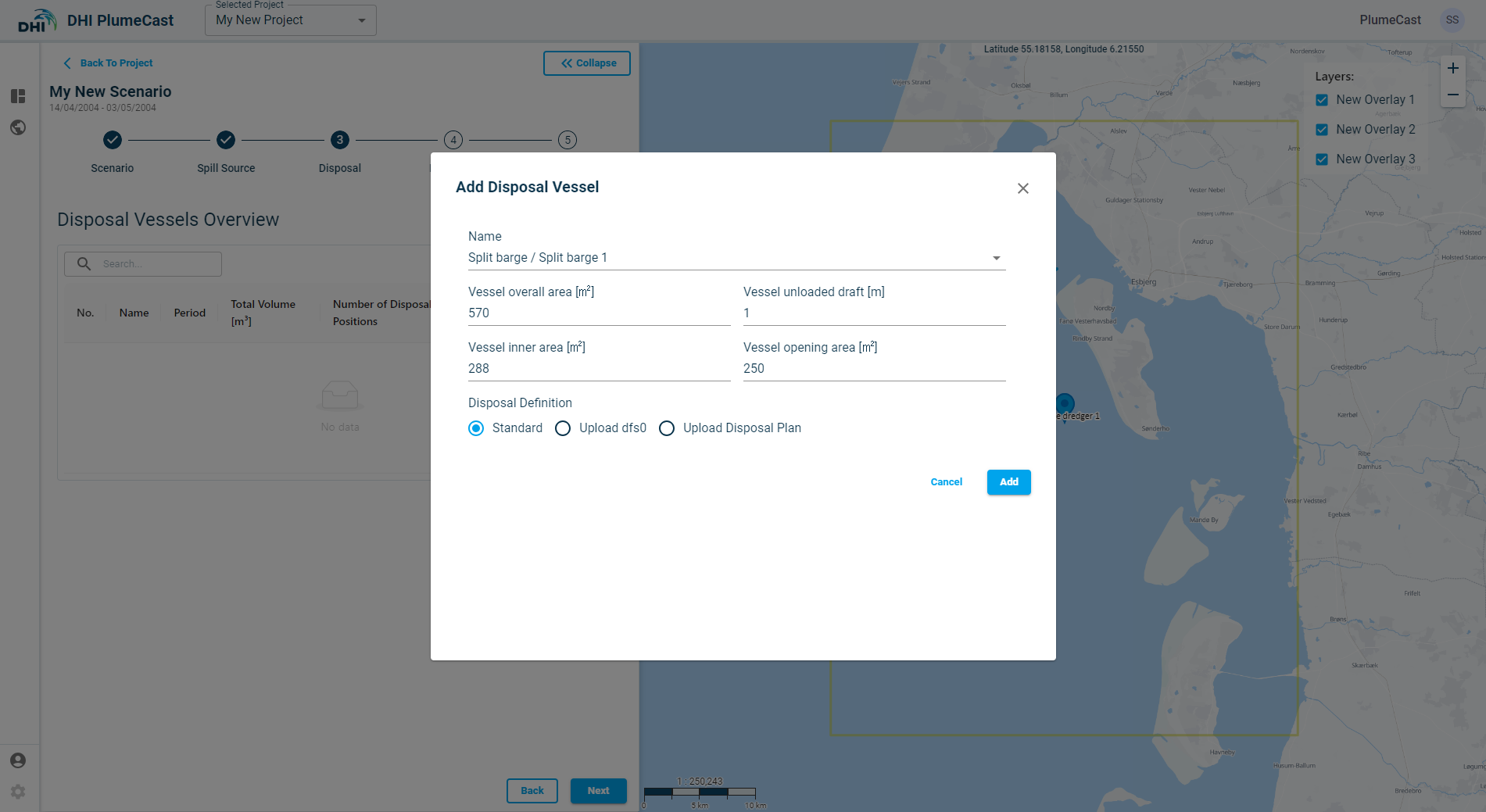
The first step is to choose the Vessel (split barge) which is doing the disposal. In the drop down you can see only the ‘Split Barge’ type of vessels only if it was defined in your project.
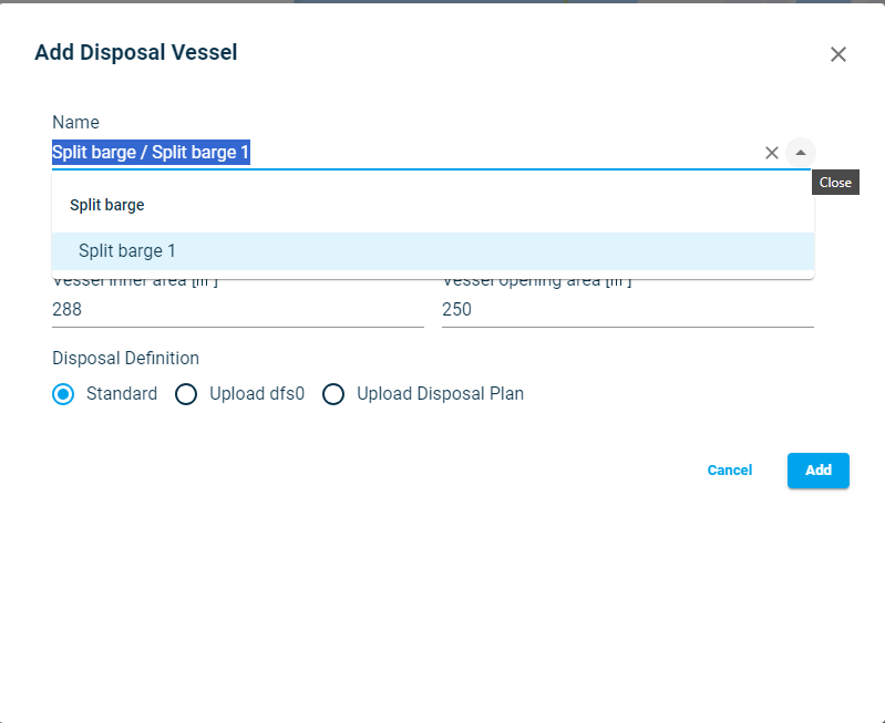
The nearfield calculator of disposal plume needs extra information regarding the dimensions of the barge. These are: - Vessel Overall area - barge inner area - barge opening area - vessel unloaded draft
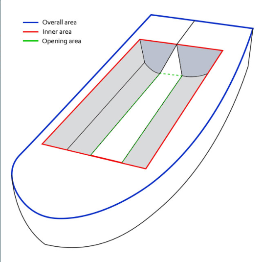
These values are retrieved from the vessel definition in the project. You can edit them, if necessary, at this stage when adding the vessel.
Next is to choose the type of disposal definition. Similar to ‘Spill Source’, the Disposal can be ‘Standard’, ‘from dfs0 file’, or ‘Disposal plan’ which is based on a csv file.
Standard Disposal definition
By choosing Standard mode, you must provide information on disposal loads and locations manually via the website. Your disposal vessel will be added to the overview list with ‘position type’ set to ‘Custom’.
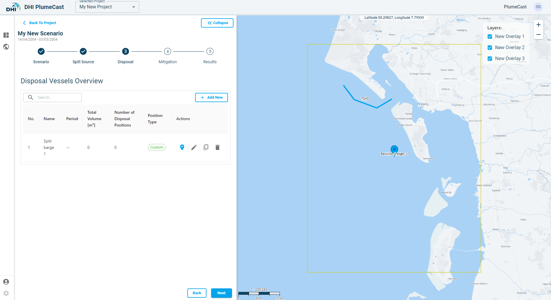
Click on the ‘location’ icon ![]() to enter the information regarding the disposal locations and its other properties.
to enter the information regarding the disposal locations and its other properties.
Note: You cannot proceed to the next step before adding at least one position for the defined Disposal.
While in the ‘Disposal Position’ page, click on ‘Add New’, a point will be added to the list and will appear on the map. The default location of the point is at the centre of the domain borders.
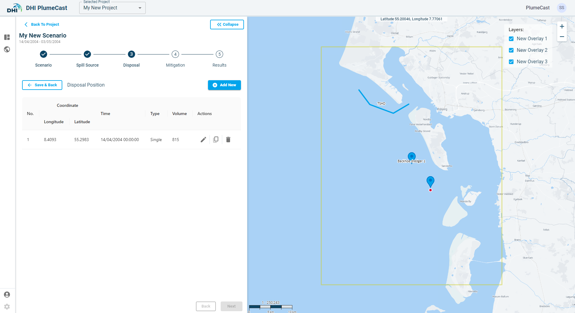
For each of the defined positions, you must provide additional information. Click on the ‘edit’ icon in front of the defined position. Here you can edit the coordinates of the point (in Longitude & Latitude), the total load volume at each disposal event (in cubic meters), the solid content of the load (in percentage between 0 and 100), distribution of different sediment fractions in the disposal load (must add up to 100), and the temperature and salinity of the water content in the disposal load. The number of fractions, their names and characteristics vary between different models and are defined during the model preparation stage.
Another way to edit the location of the disposal is by grabbing and dragging the point on the map.
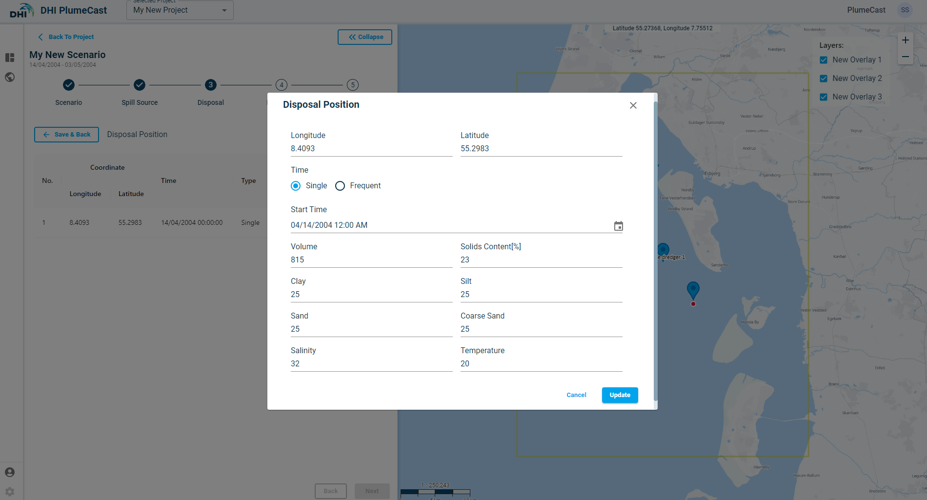
You must also define the timing of the disposal event(s) at this position point. It can be a ‘Single’ disposal event, for which you give one time instance (as shown in above image). You can only choose a time within the scenario period.
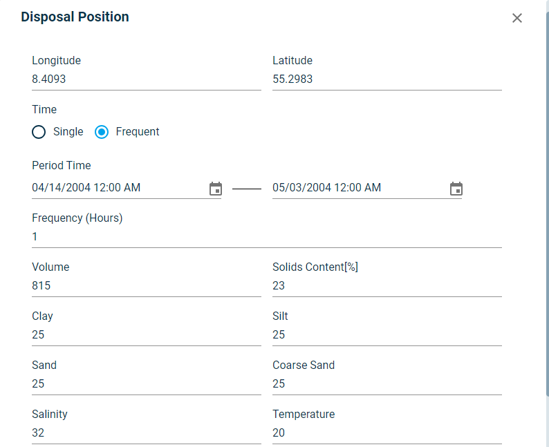
It can be frequent/recursive disposal events, for which you must define the starting, ending and the Frequency (Hours) of the disposal events. For more complex scheduling of disposal events, you must use the other two types of disposal definitions (upload dfs0 or upload csv disposal plan).
Disposal by uploading dfs0
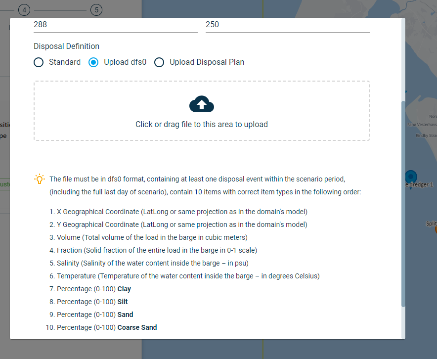
If you have prepared your disposal plan in MIKE dfs0 timeseries format, you can directly upload it to DHI PlumeCast for each disposal vessel you add in your scenario. In this case, you only need to choose the vessel. The remaining of the information are supposed to be delivered via the uploaded dfs0 file.
As seen below, the dfs0 timeseries file must include individual disposal events. It does not necessarily need to cover the entire scenario period. It must have at least one disposal event within the scenario period. It must have the following item types, and the number of items. In this example the domain’s sediment transport model was based on four sediment fractions, therefore the dfs0 file needs to have in total of 10 items.
If the dfs0 file is uploaded successfully, you will see a success message and clicking on ‘Add’ in the bottom right will add the file to the list. Your new disposal (with position type set to ‘dfs0’) will be added to the list of your disposals.
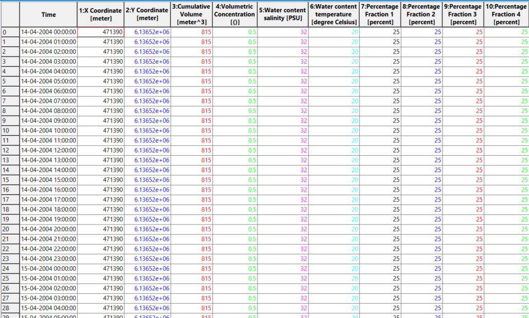
An example of a dfs0 disposal with 4 sediment fractions is shown below.
Notice that only the disposal event (when it starts) is given in the timeseries. The timeseries can be non-equidistant and only containing the disposal events.
Disposal by uploading csv Disposal plan
If you have prepared your disposal plan in csv timeseries format, you can directly upload it to DHI PlumeCast for each disposal you define in your scenario. In this case, you only need to choose the vessel. The remaining of information are supposed to be delivered via the uploaded csv file.
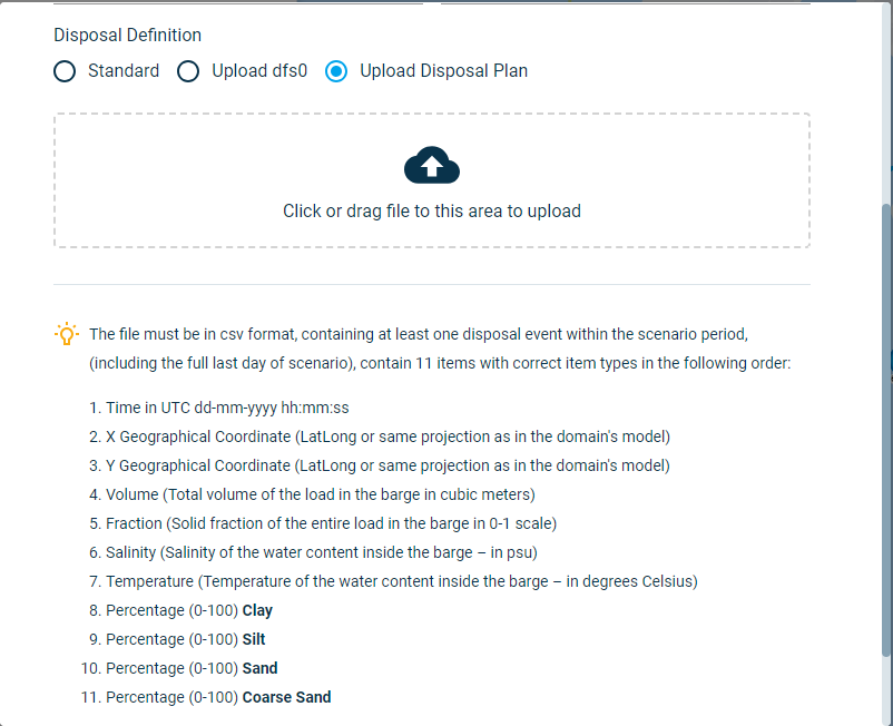
As seen below, the csv timeseries file must include individual disposal events. It does not necessarily need to cover the entire scenario period. It must have at least one disposal event within the scenario period. It must have the following columns, and the number of columns. In this example the domain’s sediment transport model was based on four sediment fractions, therefore the csv file needs to have in total of 11 columns.
If the csv file is uploaded successfully, you will see a success message and clicking on ‘Add’ in the bottom right will add the file to the list. Your new disposal (with position type set to ‘Disposal Plan’) will be added to the list of your disposals.
An example of a csv disposal with 4 sediment fractions is shown below.
Notice that only the disposal event (when it starts) is given in the timeseries.

Mitigation
In this step you can define mitigation measures against dispersion of sediment plumes. The mitigation measure currently available in DHI PlumeCast is the floating silt/turbidity curtain. It can represent any type of curtain blocking the dispersion of sediment plumes, such as curtains made out of textiles, or air bubbles.
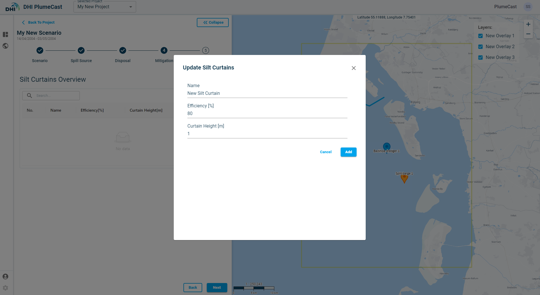
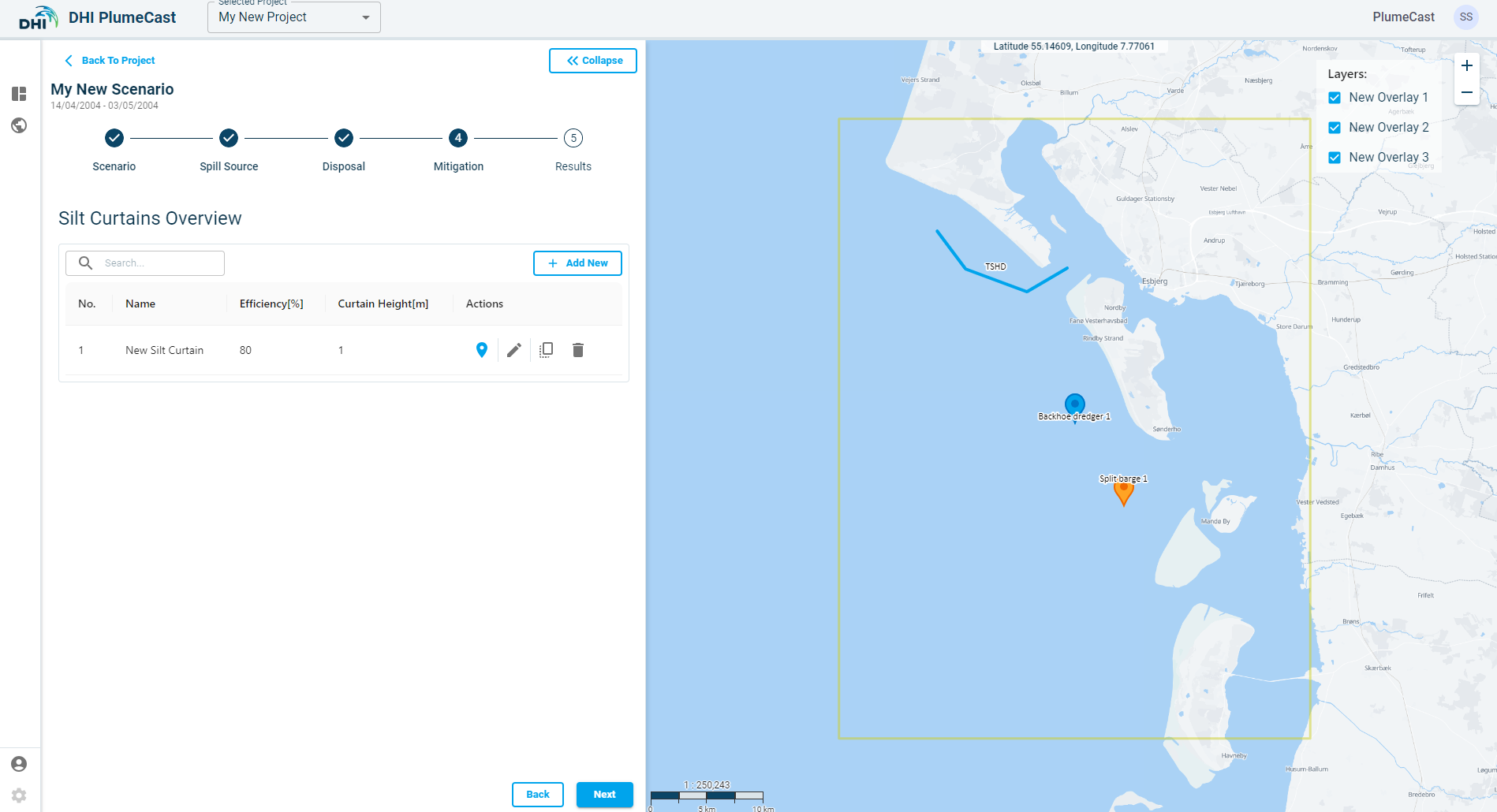
Click on ‘Add New’ to begin defining your silt curtain. You must give a name, efficiency (in percentage, between 0-100) and the curtain height.
Efficiency of the curtain represents how effective the curtain is during the scenario period. In reality, the textile curtains may tear apart, have opening in their joints or in general malfunction for any other reasons.
Similarly, the bubble curtains may not block 100% of the plume reaching them, or get weakened by currents, or vessel passage etc. All these mentioned deficiencies can be represented by the efficiency percentage given by the user here. In the MIKE model this will be translated into the percentage of the sediment/water flux being allowed to path through the curtain.
The curtain height is calculated from water surface downward. Since the curtain is floating, the given height indicates if there will be an opening between the bottom of the curtain and the seabed. This opening will vary as the water levels varies.
If you want to block the entire water column, and are not sure about the exact depth, you can give a very large number to the curtain height to assure its always larger than the local water depth. The model will ignore the extra height of the curtain beyond the water depth.
After adding the silt curtain to the overview list, you must provide its position. Currently it is only possible to define the curtains position manually on the map.
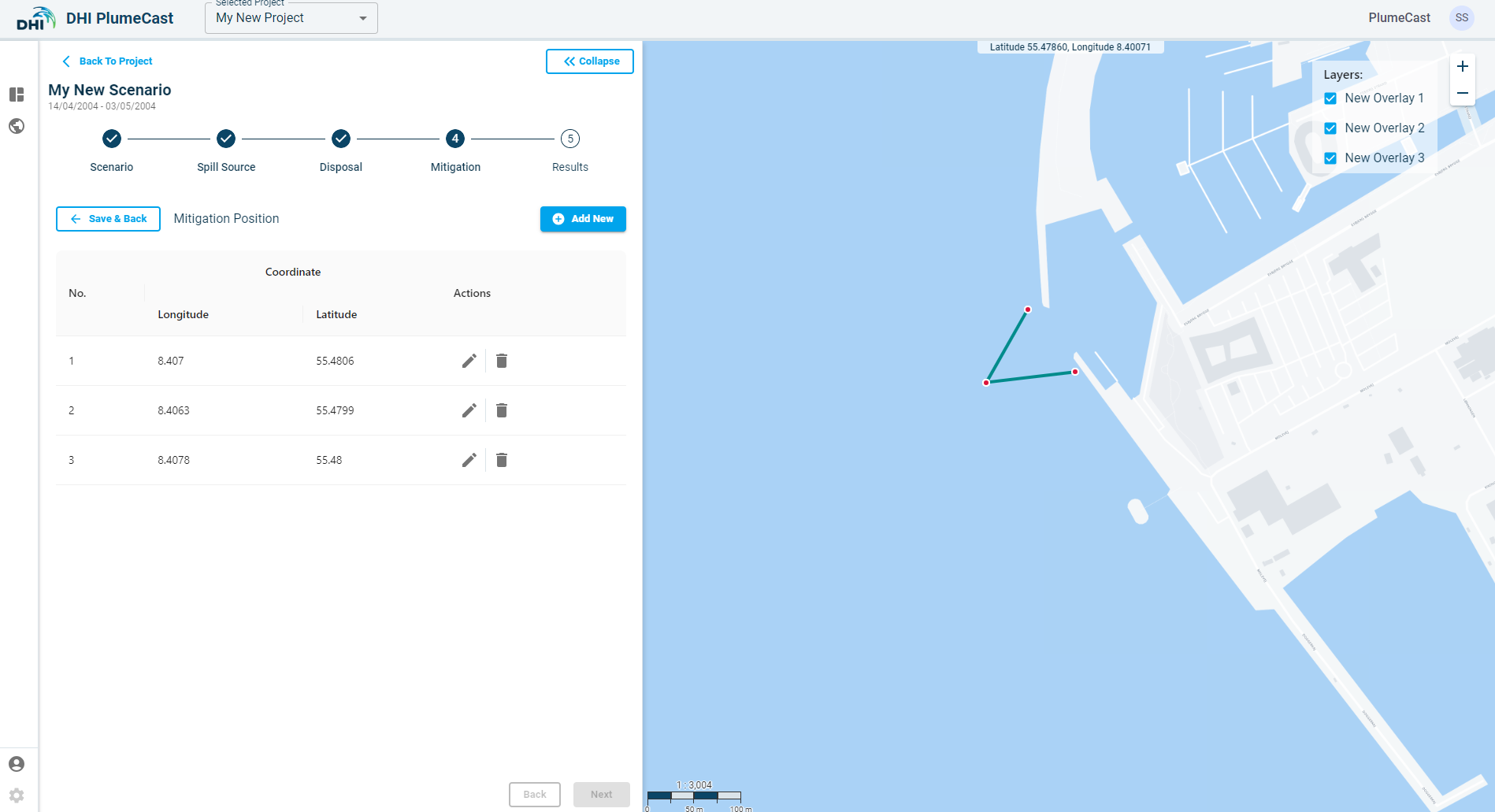
Click on the ‘position’ icon ![]() in front of the defined silt curtain and add new position points to it. The first position by default is placed at the centre of the domain borders (shown by red rectangle in the map). Silt curtains need at least two position points (to be able to define a line).
in front of the defined silt curtain and add new position points to it. The first position by default is placed at the centre of the domain borders (shown by red rectangle in the map). Silt curtains need at least two position points (to be able to define a line).
You can edit the location of the points by clicking on the ‘edit’ icon for each of the entries made, or by grabbing and dragging the points on the map.
Note: Including silt curtains in your scenario means that the hydrodynamics will be updated, hence your scenario will consume more resources and therefore it will take longer for the scenario run to complete.
Results
In this step you define and adjust the presentation and postprocessing of the Results of your scenario. You have the following parts:
- Defining extra SSC Outputs
- Defining the Statistical Analysis
- Defining timeseries extraction points from results (Monitoring Points)
- Defining timeseries extractions of discharge/flux along a line (Monitoring Lines)
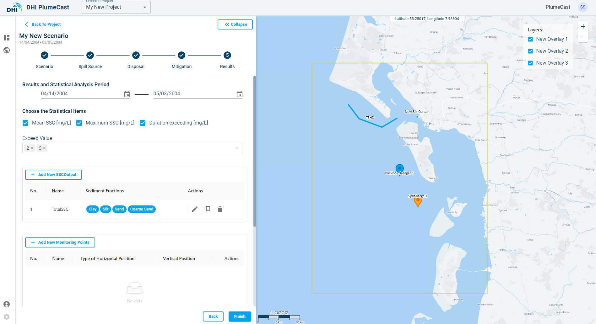
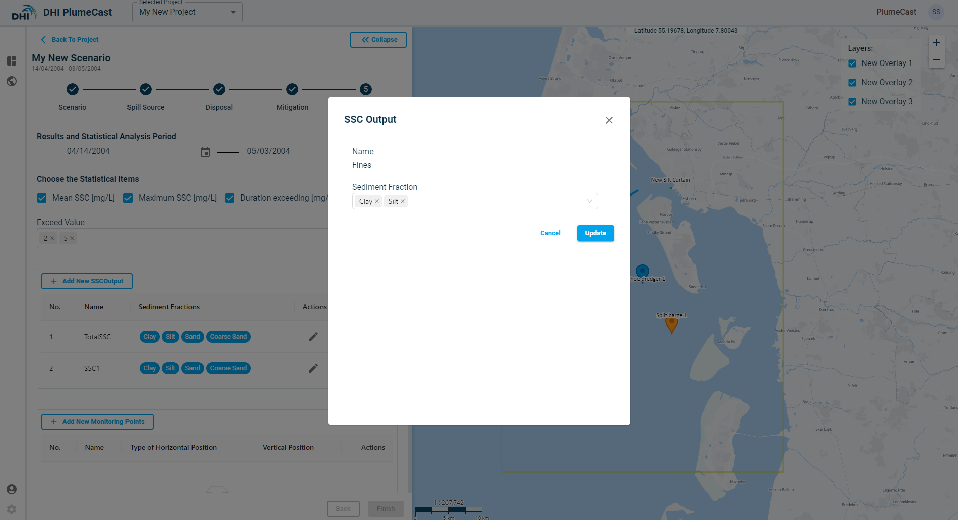
SSC Outputs
The domain model has certain number of sediment fractions defined in it. You can decide if you only want to see the Suspended Sediment Concentrations (SSC) maps of the sum of all sediment fractions, (TotalSSC), or you need to also have more combinations, for example only the first two fine fractions, or only the clay fraction, etc.
Consequently, all statistical analysis will be done for all defined SSC combinations, and when defining point timeseries extractions (Monitoring Points) or discharge lines (Monitoring lines) you can choose which SSCOutput it must be based on.
You can add as many combinations as you want in the ‘Sediment Concentration Outputs’, by clicking on ‘Add New SSC Outputs’. You can then edit them, change the name and include/exclude the fractions from them.
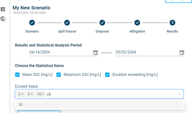
Statistical Analysis
You can choose which statistical analysis you want to be done on your scenario results, and within which period. By default, the statistical analysis is done for the entire scenario period, however you have the possibility to do them for a certain period by selecting the start and end date.
By default, we have the following statistical:
- Mean SSC: it calculates the average suspended sediment concentration over the entire model area.
- Maximum SSC: it calculates the maximum suspended sediment concentration occurred over the entire model area.
- Duration exceeding: It calculates the accumulated duration in which suspended sediment concentrations have exceeded a certain value. You can add as many exceedance values as you need. By default, there are exceedance values of 2 mg/l and 5 mg/l included. You can add more values by typing in the box and removing them by clicking on the X in front of each.
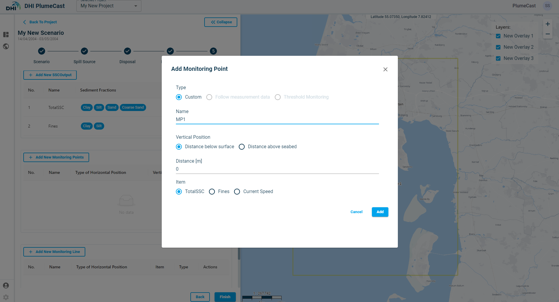
Monitoring Points
In this section you can define points within the domain, to extract from the modelling results, the timeseries of suspended sediment concentrations, or currents speeds and directions.
Click on ‘Add New Monitoring Points’. A window opens where you define the new monitoring point characteristics. Its default location will be at the centre of the border domain.
The default ‘Type’ is ‘Custom’. The ‘Follow Measurement Data’ and ‘Threshold monitoring’ type is only available if you have access to Live Data, and you have defined Measurement Points and Threshold points in the Threshold Monitoring section of Project. You can set the vertical location to extract values from the modelling results, either as ‘Distance above seabed’ or ‘Distance below surface’. If the domain’s model is a 2-dimensional model, this distance has no impact on extraction, since all model results are depth averaged. You can choose what to extract from the modelling results, by choosing either one of the SSC Outputs or ‘Current Speed’.
To edit the location of the monitoring point, click on the ‘location’ icon ![]() in front of the corresponding Monitoring point in the list to open a new window in which you can see the coordinates. You can edit the coordinates by grabbing and moving the point on map until it sits in your desired location.
in front of the corresponding Monitoring point in the list to open a new window in which you can see the coordinates. You can edit the coordinates by grabbing and moving the point on map until it sits in your desired location.
Monitoring Line
In this section you can define lines within the domain, to extract from modelling results the discharge/flux of sediments or flow through them.
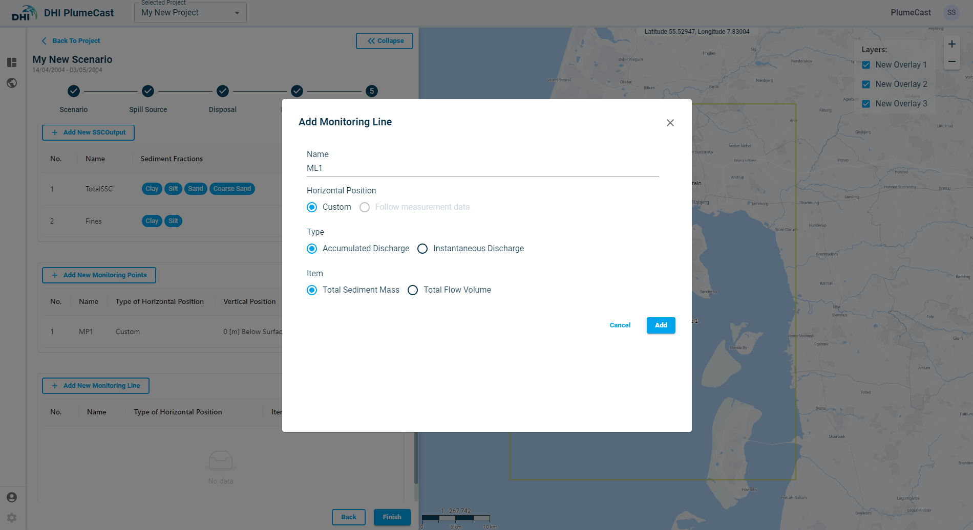
Click on ‘Add New Monitoring Lines.’ A window will open for you to define the new monitoring line characteristics.
The default ‘horizontal position’ is ‘Custom’, meaning that you set the location of the point on the map. The ‘Follow measurement data’ option is only available if you are using DHI PlumeCast with Live Data access, and DHI PlumeCast is connected to the live data from measurement data.
Two different types of information can be requested:
- Accumulated Discharge: By choosing this type, the resulting timeseries shows the total net accumulated amount of sediments (in tons) or water flow (in cubic meters) that has passed through the defined line.
- Instantaneous Discharge: By choosing this type, the resulting timeseries shows the instantaneous rate of sediment mass (in kg/sec) or water discharge (in m3/s) passing through the line at each moment.
Two different items can be extracted along the monitoring line:
- Total Sediment Mass
- Total Flow Volume
After editing and adjusting the discharge line parameters, you must define the position of the monitoring line.
Click on the ‘location’ icon ![]() in front of the defined monitoring line:
in front of the defined monitoring line:
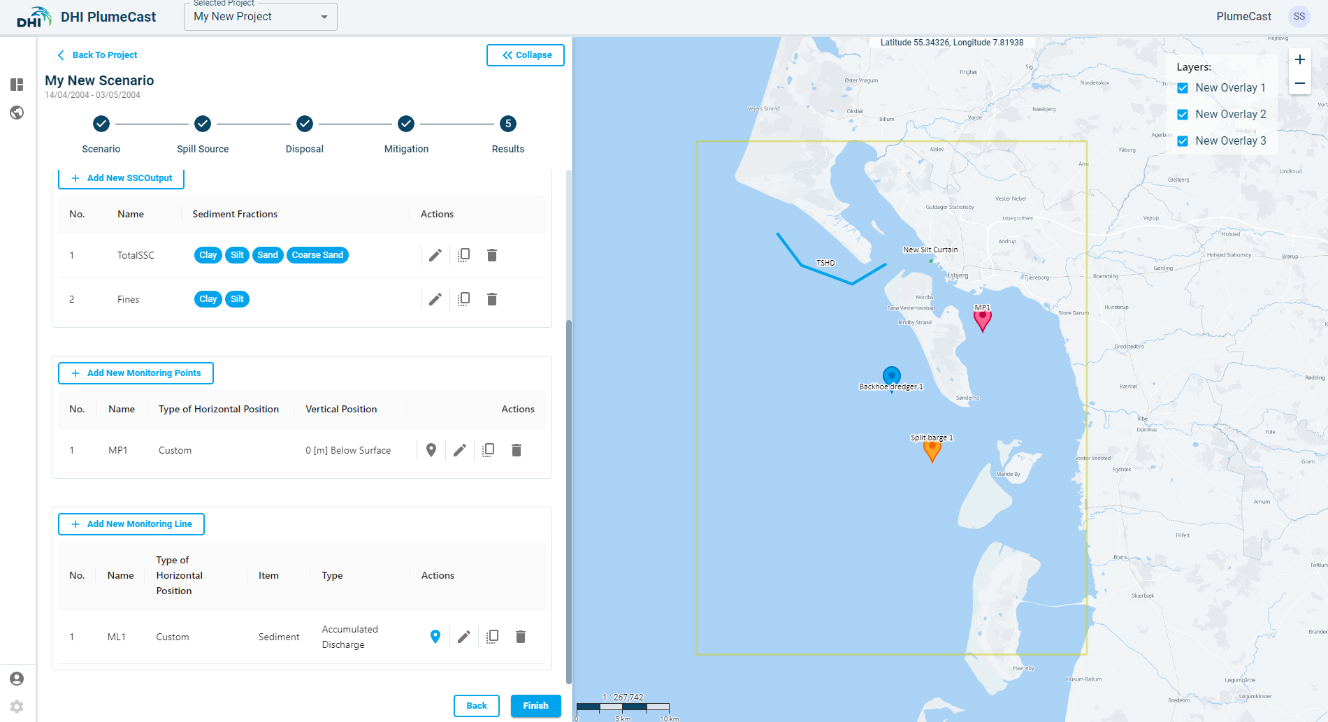
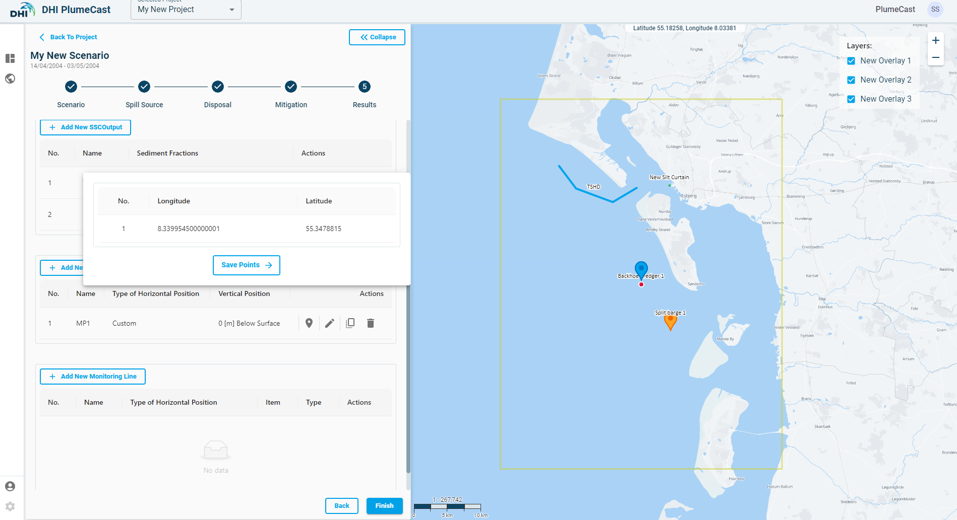
You see a new window showing an overview list of the position points for the corresponding monitoring line:
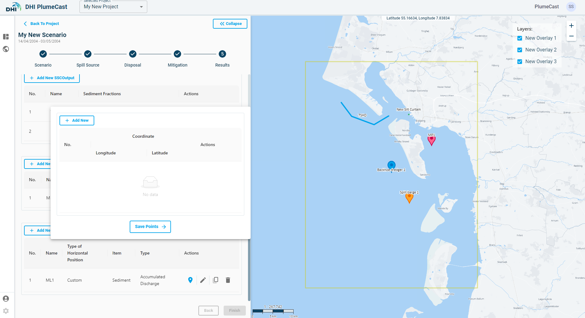
Click on ‘Add New’ to begin adding position points for your monitoring line.
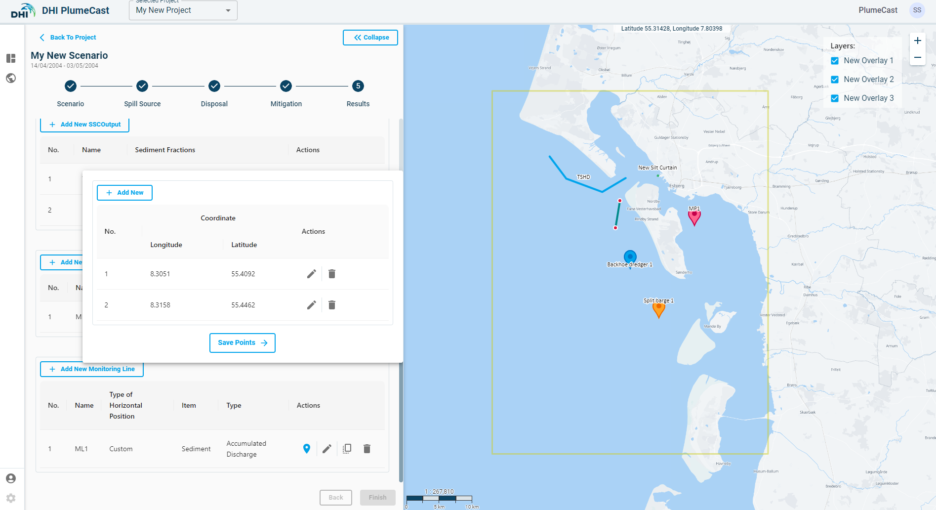
You can edit the coordinates of the points by clicking on the edit icon in front of each point in the list, or by grabbing and dragging the points on the map.
Click on ‘Save Points’ button after all the details of the location have been entered to go back to the list of monitoring points.
Note: You need at least 2 points for each monitoring line, otherwise you cannot proceed.
This is the last step in defining your scenario. After this, you can click on ‘Finish’ which will finalise the scenario definition and direct you back to the project page with scenario overview table.
Scenario execution
In the scenario overview list, you can see all the scenarios within your project. When the scenario’s status is ‘Ready’ it means it is ready to be executed. You can click the ‘Run’ button for the scenario to begin the execution.
After clicking on Run button, the scenario’s status changes to ‘In progress’. It means that the system is now reading your scenario, preparing the model files and eventually executes your scenario in MIKE. When the MIKE simulation starts, you begin to see the percentage of completion as a progress bar in scenario’s status column.
If the scenario execution finishes successfully, the scenario’s status changes to ‘Completed’. In this case, the ‘Results’ button becomes activated, and you can press on it to see the scenario results.
Scenario list:
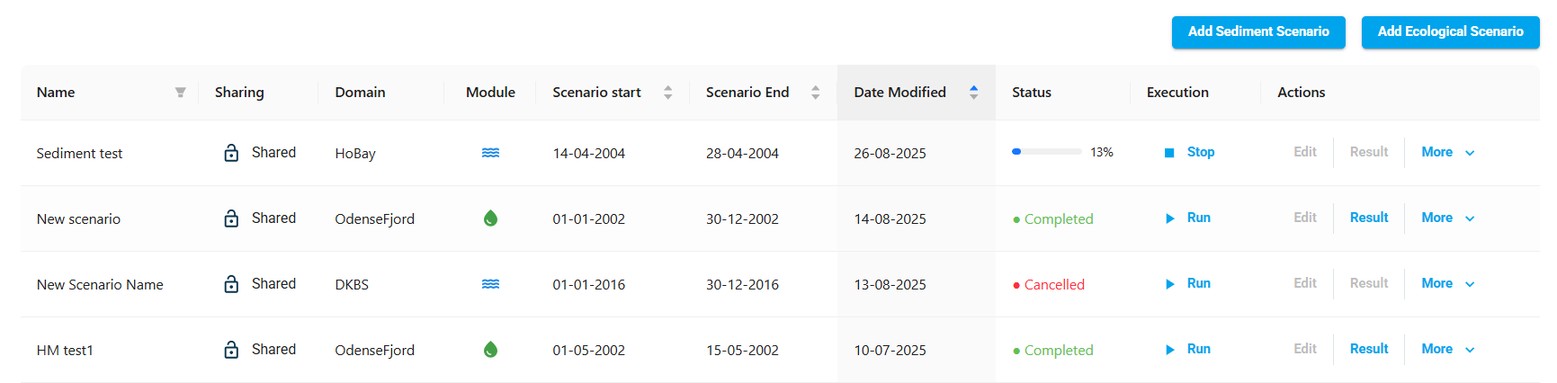
If something goes wrong and scenario execution fails, the scenario status changes to ‘Failed’.

If the scenario is running, and you want to stop it from running any further, a Stop action will appear for you to click, and the status will change to Cancelled.
